Volatility modelling: EWMA and GARCH
Contents
Volatility modelling: EWMA and GARCH#
Import the necessary packages
packages |
acronyms |
|---|---|
matplotlib.pyplot |
plt |
numpy |
np |
os |
|
pandas |
pd |
scipy.optimize |
spop |
import matplotlib.pyplot as plt
import numpy as np
import os
import pandas as pd
import scipy.optimize as spop
import warnings

warnings.simplefilter('ignore')
Set your working directory using
os.chdir([PATH])(change directory).
#os.chdir(r'C:\Users\cdes1\OneDrive - ICHEC\Documents\Cours\PortfolioManagement')
os.chdir(r'/Users/christophe/OneDrive - ICHEC/Documents/Cours/PortfolioManagement')
Check that the working directory has been updated (
os.getcwd()).
os.getcwd()
'/Users/christophe/Library/CloudStorage/OneDrive-ICHEC/Documents/Cours/PortfolioManagement'
S&P500#
Import the excel File
sp500_daily.xlsx(in yourdatafolder) as a DataFrame calleddf.
df = pd.read_excel('data/sp500_daily.xlsx', index_col=0, parse_dates=True)
Display the first 5 rows of this DataFrame (using
df.head()).
df.head()
| CLOSE | |
|---|---|
| Date | |
| 1930-01-02 | 21.18 |
| 1930-01-03 | 21.23 |
| 1930-01-04 | 21.48 |
| 1930-01-06 | 21.50 |
| 1930-01-07 | 21.31 |
Display the last 5 rows of this DataFrame (using
df.tail()).
df.tail()
| CLOSE | |
|---|---|
| Date | |
| 2022-12-23 | 3844.8150 |
| 2022-12-27 | 3829.2493 |
| 2022-12-28 | 3783.2219 |
| 2022-12-29 | 3849.2832 |
| 2022-12-30 | 3839.4966 |
Display some information about this DataFrame (using
df.info()).
df.info()
<class 'pandas.core.frame.DataFrame'>
DatetimeIndex: 24060 entries, 1930-01-02 to 2022-12-30
Data columns (total 1 columns):
 #   Column  Non-Null Count  Dtype
---  ------  --------------  -----
 0   CLOSE   24060 non-null  float64
dtypes: float64(1)
memory usage: 375.9 KB
Rename the column “CLOSE” as “price”.
https://pandas.pydata.org/docs/reference/api/pandas.DataFrame.rename.html
df.rename(columns={'CLOSE': 'price'}, inplace=True)
df
| price | |
|---|---|
| Date | |
| 1930-01-02 | 21.1800 |
| 1930-01-03 | 21.2300 |
| 1930-01-04 | 21.4800 |
| 1930-01-06 | 21.5000 |
| 1930-01-07 | 21.3100 |
| ... | ... |
| 2022-12-23 | 3844.8150 |
| 2022-12-27 | 3829.2493 |
| 2022-12-28 | 3783.2219 |
| 2022-12-29 | 3849.2832 |
| 2022-12-30 | 3839.4966 |
24060 rows × 1 columns
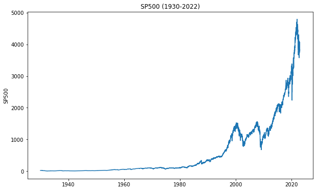
Line chart#
Create a line plot of the S&P500.
Set a label SP500 on the y-axis and a title (e.g., ’SP500 (1930-2022)’)
https://matplotlib.org/stable/gallery/index.html
Save this figure in your folder images.
fig, ax = plt.subplots(figsize=(10, 6))
ax.plot(df['price'])
# ax.plot(df) also works because there is only one column in the DataFrame
plt.ylabel('SP500')
plt.title('SP500 (1930-2022)')
fig.savefig('images/volatility_sp500.png')
plt.show()
Compute the logarithmic returns.
Remove the first missing row.
Rename the column “price” into “rets”
Display the first 5 rows.
rets = np.log(df / df.shift(1)).dropna() # rendement log
rets.rename(columns={'price': 'rets'}, inplace=True)
rets.head()
| rets | |
|---|---|
| Date | |
| 1930-01-03 | 0.002358 |
| 1930-01-04 | 0.011707 |
| 1930-01-06 | 0.000931 |
| 1930-01-07 | -0.008876 |
| 1930-01-08 | -0.000939 |
Compute the volatility
“Classical formula”: Volatility is computed as the standard deviation of the returns. To annualize volatility, multiply by the square root of data frequency.
historical_volatility = np.std(rets) * np.sqrt(252)
historical_volatility
rets    0.182536
dtype: float64
Note: the [0] is needed in order to only get the number.
historical_volatility = np.std(rets) * np.sqrt(252)
historical_volatility
rets    0.182536
dtype: float64
We can also use [‘rets’].
historical_volatility = np.std(rets) * np.sqrt(252)
historical_volatility['rets']
0.1825362035297431
Alternatively, we can use the .std() method on the DataFrame.
rets.std() * np.sqrt(252)
rets    0.18254
dtype: float64
Finally, a nice output, we can use format.
historical_volatility = np.std(rets) * np.sqrt(252)
historical_volatility = historical_volatility['rets']
print("{:.4%}".format(historical_volatility))
18.2536%
“Finance formula”: We can also make the simplifying assumption that \(\bar{r} = 0\). In this case, the variance is simply the sum of the squared returns.
historical_volatility = np.sqrt(np.mean(rets**2, axis=0)) * np.sqrt(252)
historical_volatility = historical_volatility[0]
print("{:.4%}".format(historical_volatility))
18.2568%
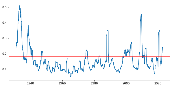
Rolling volatility
Volatility is not constant. Let’s compute it and plot it using a rolling window of 252 days (approximately 1 year).
rolling_vol = (rets.rolling(252).std()*np.sqrt(252))
fig, ax = plt.subplots(figsize=(10,5))
ax.plot(rolling_vol)
plt.axhline(historical_volatility, color='red')
plt.savefig('images/volatility_rolling_window_volatility.png')
plt.show();
EWMA#
Using the returns from 2010, use the EWMA to model volatility
To make things visual, we will put everything inside the DataFrame, very similar to what we would have done in Excel.
rets = rets.loc['2010-01-01':].copy()
rets.head()
| rets | |
|---|---|
| Date | |
| 2010-01-04 | 0.015910 |
| 2010-01-05 | 0.003118 |
| 2010-01-06 | 0.000540 |
| 2010-01-07 | 0.004000 |
| 2010-01-08 | 0.002876 |
Compute the number of observations and store this value in n.
n = rets.shape[0]
n
3272
Compute the squared returns and store it in a new column rets_sq.
rets['rets_sq'] = rets['rets']**2
rets
| rets | rets_sq | |
|---|---|---|
| Date | ||
| 2010-01-04 | 0.015910 | 2.531178e-04 |
| 2010-01-05 | 0.003118 | 9.720487e-06 |
| 2010-01-06 | 0.000540 | 2.920861e-07 |
| 2010-01-07 | 0.004000 | 1.599607e-05 |
| 2010-01-08 | 0.002876 | 8.271171e-06 |
| ... | ... | ... |
| 2022-12-23 | 0.005850 | 3.422799e-05 |
| 2022-12-27 | -0.004057 | 1.645688e-05 |
| 2022-12-28 | -0.012093 | 1.462353e-04 |
| 2022-12-29 | 0.017311 | 2.996689e-04 |
| 2022-12-30 | -0.002546 | 6.480512e-06 |
3272 rows × 2 columns
Create a vector conditional of zero’s with size n and add this vector in a column conditional.
conditional = np.zeros(n)
rets['conditional'] = conditional
rets
| rets | rets_sq | conditional | |
|---|---|---|---|
| Date | |||
| 2010-01-04 | 0.015910 | 2.531178e-04 | 0.0 |
| 2010-01-05 | 0.003118 | 9.720487e-06 | 0.0 |
| 2010-01-06 | 0.000540 | 2.920861e-07 | 0.0 |
| 2010-01-07 | 0.004000 | 1.599607e-05 | 0.0 |
| 2010-01-08 | 0.002876 | 8.271171e-06 | 0.0 |
| ... | ... | ... | ... |
| 2022-12-23 | 0.005850 | 3.422799e-05 | 0.0 |
| 2022-12-27 | -0.004057 | 1.645688e-05 | 0.0 |
| 2022-12-28 | -0.012093 | 1.462353e-04 | 0.0 |
| 2022-12-29 | 0.017311 | 2.996689e-04 | 0.0 |
| 2022-12-30 | -0.002546 | 6.480512e-06 | 0.0 |
3272 rows × 3 columns
Initialize the second value as the squared value of the first return.
# rets.iloc[1]['conditional'] = rets.iloc[0]['rets']**2
# this results in a warning
rets.loc[rets.index[1], 'conditional'] = rets.iloc[0]['rets_sq']
rets
| rets | rets_sq | conditional | |
|---|---|---|---|
| Date | |||
| 2010-01-04 | 0.015910 | 2.531178e-04 | 0.000000 |
| 2010-01-05 | 0.003118 | 9.720487e-06 | 0.000253 |
| 2010-01-06 | 0.000540 | 2.920861e-07 | 0.000000 |
| 2010-01-07 | 0.004000 | 1.599607e-05 | 0.000000 |
| 2010-01-08 | 0.002876 | 8.271171e-06 | 0.000000 |
| ... | ... | ... | ... |
| 2022-12-23 | 0.005850 | 3.422799e-05 | 0.000000 |
| 2022-12-27 | -0.004057 | 1.645688e-05 | 0.000000 |
| 2022-12-28 | -0.012093 | 1.462353e-04 | 0.000000 |
| 2022-12-29 | 0.017311 | 2.996689e-04 | 0.000000 |
| 2022-12-30 | -0.002546 | 6.480512e-06 | 0.000000 |
3272 rows × 3 columns
Initialize a variable lambda_val with a value of 0.94. Then, implement this formula:
Note 1: lambda cannot be used as variable name as it has another signification in Python.
Note 2: the vector rets has one additional observation in comparison to the vector conditional.
lambda_val = 0.94

for t in range(2, n):
    rets.loc[rets.index[t], 'conditional'] = lambda_val * rets.iloc[t-1]['conditional'] \
                                             + (1 - lambda_val) * rets.iloc[t-1]['rets'] ** 2

rets.head()
| rets | rets_sq | conditional | |
|---|---|---|---|
| Date | |||
| 2010-01-04 | 0.015910 | 2.531178e-04 | 0.000000 |
| 2010-01-05 | 0.003118 | 9.720487e-06 | 0.000253 |
| 2010-01-06 | 0.000540 | 2.920861e-07 | 0.000239 |
| 2010-01-07 | 0.004000 | 1.599607e-05 | 0.000224 |
| 2010-01-08 | 0.002876 | 8.271171e-06 | 0.000212 |
Compute the loglikelihood as:
where:
\(u_i\): return
\(v_i\): conditional
rets.loc[rets.index[1:], 'likelihood'] = -np.log(rets.iloc[1:]['conditional']) \
                                         -((rets.iloc[1:]['rets']**2)/rets.iloc[1:]['conditional'])
rets.head()
| rets | rets_sq | conditional | likelihood | |
|---|---|---|---|---|
| Date | ||||
| 2010-01-04 | 0.015910 | 2.531178e-04 | 0.000000 | NaN |
| 2010-01-05 | 0.003118 | 9.720487e-06 | 0.000253 | 8.243253 |
| 2010-01-06 | 0.000540 | 2.920861e-07 | 0.000239 | 8.339858 |
| 2010-01-07 | 0.004000 | 1.599607e-05 | 0.000224 | 8.331539 |
| 2010-01-08 | 0.002876 | 8.271171e-06 | 0.000212 | 8.421147 |
Compute the sum of the log-likelihood into log_likelihood.
log_likelihood = rets['likelihood'].sum()
log_likelihood
27407.697995474882
Wrap everything within a function ewma_pandas, which takes two arguments: (1) the value of the lambda (lambda_val) and (2) the returns. This function returns the value of the loglikelihood.
def ewma_pandas(lambda_val, rets):
    df = rets.copy()
    n = df.shape[0]
    df['rets_sq'] = df['rets']**2
    conditional = np.zeros(n)
    df['conditional'] = conditional
    df.loc[df.index[1], 'conditional'] = df.iloc[0]['rets']**2
    for t in range(2, n):
        df.loc[df.index[t], 'conditional'] = lambda_val * df.iloc[t-1]['conditional'] \
                                             + (1 - lambda_val) * df.iloc[t-1]['rets'] ** 2
    df.loc[df.index[1:], 'likelihood'] = -np.log(df.iloc[1:]['conditional']) \
                                         -((df.iloc[1:]['rets']**2)/df.iloc[1:]['conditional'])
    log_likelihood = df['likelihood'].sum()
    return -log_likelihood
df = pd.read_excel('data/sp500_daily.xlsx', index_col=0, parse_dates=True)
rets = np.log(df/df.shift(1)).dropna()
rets.rename(columns={'CLOSE':'rets'}, inplace=True)
rets = rets.loc['2010-01-01':]
rets
| rets | |
|---|---|
| Date | |
| 2010-01-04 | 0.015910 |
| 2010-01-05 | 0.003118 |
| 2010-01-06 | 0.000540 |
| 2010-01-07 | 0.004000 |
| 2010-01-08 | 0.002876 |
| ... | ... |
| 2022-12-23 | 0.005850 |
| 2022-12-27 | -0.004057 |
| 2022-12-28 | -0.012093 |
| 2022-12-29 | 0.017311 |
| 2022-12-30 | -0.002546 |
3272 rows × 1 columns
Call this function with a lambda value of 0.94. You should find the same value.
rets

ewma_pandas(0.94, rets)
-27407.697995474882
Naive optimization#
For different values of lambda between 0.80 and 1.00, compute the value of the different loglikelihood and plot it.
lambda_vals = np.arange(0.80, 1, 0.005)
log_vals = [-ewma_pandas(lam, rets) for lam in lambda_vals]
plt.plot(lambda_vals, log_vals);
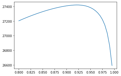
We notice a maximum around 0.925. Let’s now optimize it to find the actual answer.
# reinitialize dataframe
rets = np.log(df / df.shift(1)).dropna() # rendement log
rets.rename(columns={'CLOSE': 'rets'}, inplace=True)
rets = rets.loc['2010-01-01':].copy()

var = np.std(rets)**2 # historical variance
res = spop.minimize(ewma_pandas, var, rets, method="Nelder-Mead")
params = res.x
function = res.fun
print('Parameters: ', res.x)
print('LogLikelihood: ', -res.fun)
Parameters:  [0.92171991]
LogLikelihood:  27420.928807446242
lambda_val = res.x
df = rets.copy()
n = df.shape[0]
df['rets_sq'] = df['rets']**2
conditional = np.zeros(n)
df['conditional'] = conditional
df.loc[df.index[1], 'conditional'] = df.iloc[0]['rets']**2
for t in range(2, n):
    df.loc[df.index[t], 'conditional'] = lambda_val * df.iloc[t-1]['conditional'] \
                                         + (1 - lambda_val) * df.iloc[t-1]['rets'] ** 2
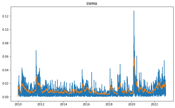
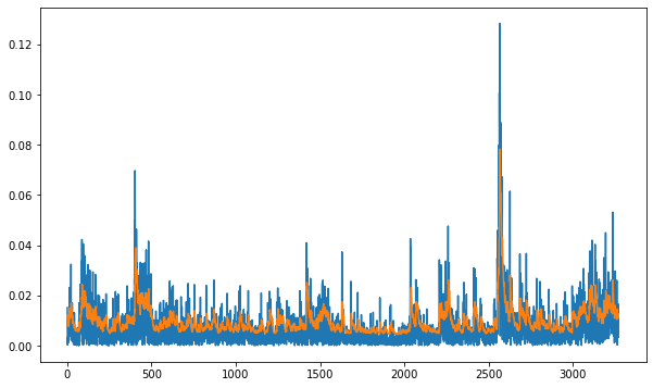
fig, ax = plt.subplots(figsize=(10,6))
ax.plot(np.abs(df['rets']))
ax.plot(df['conditional']**(1/2))
ax.set_title('EWMA')
plt.show()
%%time

ewma_pandas(0.94, rets)
CPU times: user 447 ms, sys: 1.57 ms, total: 449 ms
Wall time: 448 ms
-27407.697995474882
Improve performance using numpy#
It is not easy nor efficient to fill a DataFrame. A better approach (although less beautiful) is to work with numpy arrays. Reimplement everything without using Pandas.
df = pd.read_excel('data/sp500_daily.xlsx', index_col=0, parse_dates=True)
rets = np.log(df / df.shift(1)).dropna() # rendement log
rets.rename(columns={'CLOSE': 'rets'}, inplace=True)
rets = rets.loc['2010-01-01':]
rets = np.array(rets).ravel()
rets.shape
rets
array([ 0.01590968,  0.00311777,  0.00054045, ..., -0.01209278,
        0.01731095, -0.00254568])
n = len(rets)
n
3272
conditional = np.zeros(n-1)
conditional[0] = rets[0]**2
conditional
array([0.00025312, 0.        , 0.        , ..., 0.        , 0.        ,
       0.        ])
lambda_val = 0.94

for t in range(1, len(conditional)):
    conditional[t] = lambda_val * conditional[t-1] + (1 - lambda_val) * rets[t] ** 2

conditional
array([0.00025312, 0.00023851, 0.00022422, ..., 0.00017394, 0.00017228,
       0.00017992])
likelihood = -np.log(conditional)-((rets[1:]**2)/conditional)
likelihood
array([8.24325261, 8.33985817, 8.33153924, ..., 7.81607462, 6.92696348,
       8.58695739])
log_likelihood = np.sum(likelihood)
log_likelihood
27407.697995474882
It’s now time to wrap everything within a function ewma. We assume that we pass to the function two arguments:
the value of the lambda
a series of return in a ndarray
rets = np.array(rets)
def ewma_numpy(lambda_val, rets):
    n = len(rets)
    conditional = np.zeros(n-1)
    conditional[0] = rets[0]**2
    for t in range(1, len(conditional)):
        conditional[t] = lambda_val * conditional[t-1] + (1 - lambda_val) * rets[t] ** 2
    likelihood = -np.log(conditional)-((rets[1:]**2)/conditional)
    log_likelihood = np.sum(likelihood)
    return -log_likelihood
Let’s check we get the same value of the logLikelihood using the function.
%%time

ewma_numpy(lambda_val=0.94, rets=rets)
CPU times: user 2.42 ms, sys: 269 µs, total: 2.69 ms
Wall time: 2.49 ms
-27407.697995474882
It’s now time to optimize the function using spop.minimize.
var = np.std(rets)**2 # historical variance
res = spop.minimize(ewma_numpy, [var], rets, method="Nelder-Mead")
params = res.x
function = res.fun
print('Parameters: ', res.x)
print('LogLikelihood: ', -res.fun)
Parameters:  [0.92171991]
LogLikelihood:  27420.928807446242
GARCH Modelling (NEDL)#
Now it’s your turn to implement the GARCH method.
df = pd.read_excel('data/sp500_daily.xlsx', index_col=0, parse_dates=True)
rets = np.log(df / df.shift(1)).dropna()
rets.rename(columns={'CLOSE': 'rets'}, inplace=True)
rets = rets.loc['2010-01-01':].copy()
rets = np.array(rets)
rets = rets.ravel()
mean = np.average(rets)
var = np.var(rets)
def garch_nedl(params):
    mu = params[0]
    omega = params[1]
    alpha = params[2]
    beta = params[3]
    long_run = (omega/(1-alpha-beta))**(1/2)
    resid = rets - mu
    realised = abs(resid)
    conditional = np.zeros(len(rets))
    conditional[0] = long_run
    for t in range(1, len(rets)):
        conditional[t] = (omega + alpha*resid[t-1]**2 + beta*conditional[t-1]**2)**(1/2)
    likelihood = 1/((2*np.pi)**(1/2)*conditional)*np.exp(-realised**2/(2*conditional**2))
    log_likelihood = np.sum(np.log(likelihood))
    return -log_likelihood
#bnds = tuple((0,1) for x in range(4))
res = spop.minimize(garch_nedl, [mean, var, 0, 0],
                    #bounds=bnds,
                    method='Nelder-Mead')
params = res.x
mu = params[0]
omega = params[1]
alpha = params[2]
beta = params[3]
long_run = (omega/(1-alpha-beta))**(1/2)
resid = rets - mu
realised = abs(resid)
conditional = np.zeros(len(rets))
conditional[0] = long_run
for t in range(1, len(rets)):
    conditional[t] = (omega + alpha*resid[t-1]**2 + beta*conditional[t-1]**2)**(1/2)

print('GARCH model parameters')
print('----------------------')
print('mu', str(round(mu, 6)))
print('omega', str(round(omega, 6)))
print('alpha', str(round(alpha, 6)))
print('beta', str(round(beta, 6)))
GARCH model parameters
----------------------
mu 0.000775
omega 4e-06
alpha 0.178418
beta 0.793665
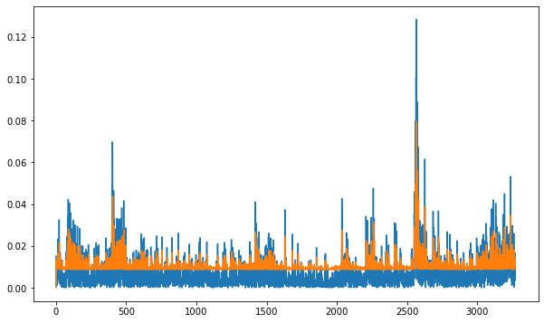
fig, ax = plt.subplots(figsize=(10, 6))
ax.plot(realised)
ax.plot(conditional)
[<matplotlib.lines.Line2D at 0x7fb3d8e45580>]
Garch zero-mean#
def garch_zero_mean(params):
    # specifying model parameters
    mu = 0
    omega = params[0]
    alpha = params[1]
    beta = params[2]
    # calculating long run volatility
    # long_run = (omega/(1 - alpha - beta))**(1/2)
    # calculating realized and conditional volatility
    resid = rets - mu
    realized = abs(resid)
    conditional = np.zeros(len(rets))
    conditional[0] = rets[0]**2
    for t in range(1, len(rets)):
        conditional[t] = (omega + alpha*resid[t-1]**2 + beta*conditional[t-1])
    # calculating loglikelihood
    likelihood = -np.log(conditional) - realized**2 / conditional
    log_likelihood = np.sum(likelihood)
    return -log_likelihood
#mean = np.average(returns)
var = np.std(rets)**2
bounds = [(0.0, 1.0)]*3
res = spop.minimize(garch_zero_mean, [var, 0, 0], bounds=bounds, method='Nelder-Mead')
mu = 0
omega = res.x[0]
alpha = res.x[1]
beta = res.x[2]
log_likelihood = -float(res.fun)
# calculating realized and conditional volatility
# long_run = (omega/(1 - alpha - beta))**(1/2)
resid = rets - mu
realized = abs(resid)
conditional = np.zeros(len(rets))
conditional[0] = rets[0]**2
for t in range(1, len(rets)):
    conditional[t] = (omega + alpha*resid[t-1]**2 + beta*conditional[t-1]**2)**(1/2)

likelihood = -np.log(conditional) - realized**2 / conditional
log_likelihood = np.sum(likelihood)

print('GARCH model parameters')
print('----------------------')
print('mu', str(round(mu, 6)))
print('omega', str(round(omega, 6)))
print('alpha', str(round(alpha, 6)))
print('beta', str(round(beta, 6)))
# print('long-run volatility', str(round(long_run, 4)))
print('log-likelihood', str(round(log_likelihood, 4)))
GARCH model parameters
----------------------
mu 0
omega 7.7e-05
alpha 0.385073
beta 0.0
log-likelihood 14968.3621
fig, ax = plt.subplots(figsize=(10, 6))
ax.plot(realised)
ax.plot(conditional)
[<matplotlib.lines.Line2D at 0x7fb3d8cddf70>]
ARCH package#
https://arch.readthedocs.io/en/latest/index.html
# !pip install arch
from arch import arch_model
am = arch_model(rets*100)
res = am.fit()
print(res.summary())
Iteration:      1,   Func. Count:      6,   Neg. LLF: 45190.138944107726
Iteration:      2,   Func. Count:     17,   Neg. LLF: 19000.159297830152
Iteration:      3,   Func. Count:     27,   Neg. LLF: 6719.894415448125
Iteration:      4,   Func. Count:     34,   Neg. LLF: 8186.897239907136
Iteration:      5,   Func. Count:     40,   Neg. LLF: 4525.832689694671
Iteration:      6,   Func. Count:     47,   Neg. LLF: 4243.099399974918
Iteration:      7,   Func. Count:     53,   Neg. LLF: 4241.2416896886125
Iteration:      8,   Func. Count:     58,   Neg. LLF: 4241.24076531225
Iteration:      9,   Func. Count:     63,   Neg. LLF: 4241.240763542724
Iteration:     10,   Func. Count:     67,   Neg. LLF: 4241.240763542601
Optimization terminated successfully    (Exit mode 0)
            Current function value: 4241.240763542724
            Iterations: 10
            Function evaluations: 67
            Gradient evaluations: 10
                     Constant Mean - GARCH Model Results
==============================================================================
Dep. Variable:                      y   R-squared:                       0.000
Mean Model:             Constant Mean   Adj. R-squared:                  0.000
Vol Model:                      GARCH   Log-Likelihood:               -4241.24
Distribution:                  Normal   AIC:                           8490.48
Method:            Maximum Likelihood   BIC:                           8514.85
                                        No. Observations:                 3272
Date:                Thu, Apr 06 2023   Df Residuals:                     3271
Time:                        16:11:37   Df Model:                            1
                                Mean Model
==========================================================================
                 coef    std err          t      P>|t|    95.0% Conf. Int.
--------------------------------------------------------------------------
mu             0.0776  1.326e-02      5.857  4.708e-09 [5.166e-02,  0.104]
                              Volatility Model
============================================================================
                 coef    std err          t      P>|t|      95.0% Conf. Int.
----------------------------------------------------------------------------
omega          0.0369  7.769e-03      4.744  2.100e-06 [2.163e-02,5.208e-02]
alpha[1]       0.1801  2.365e-02      7.616  2.609e-14     [  0.134,  0.226]
beta[1]        0.7932  2.206e-02     35.960 3.542e-283     [  0.750,  0.836]
============================================================================

Covariance estimator: robust
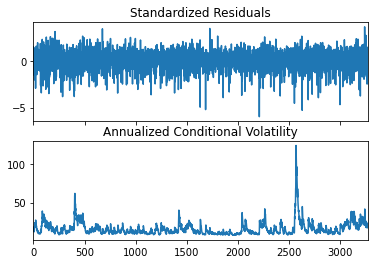
fig = res.plot(annualize="D")
References and further ressources#
NEDL - ARCH model - volatility persistence in time series (Excel)
https://www.youtube.com/watch?v=-G5g3ChktEs
NEDL - GARCH model - volatility persistence in time series (Excel)
https://www.youtube.com/watch?v=88oOzPFVWTU
NEDL - GARCH model in Python